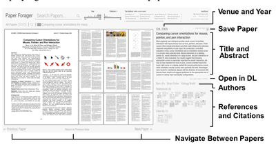
Graph Survey Likert UI Labelled UI Arrows Flow Diagram Hero Newest first Oldest first Title A–Z First author only Group by paper Size: × ‹ › View paper →

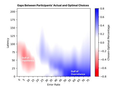
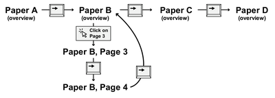
![Figure 6: Four plots illustrating the main patterns of chosen versus optimal percentages of using Assisted Fill given various error rate conditions. The y-axis in each chart represents the percentage of participants choosing Assisted Fill, with y = 1 meaning everyone chose Assisted Fill and y = 0 indicating no one chose Assisted Fill. The x-axis represents the different latency conditions. The charts represent these variables for increasing error rates: 0% (top left), 20% (top right), 50% (bottom left), and 75% (bottom right). Sigmoid curves are fitted to the raw data to illustrate trends. Shaded areas around the red and blue curves represent 1-sigma bootstrap confidence intervals [8, 40].](/publication/to-use-or-not-to-use-impatience-and/figure-6-cropped_hu_6d2d599fbfbf2329.png)
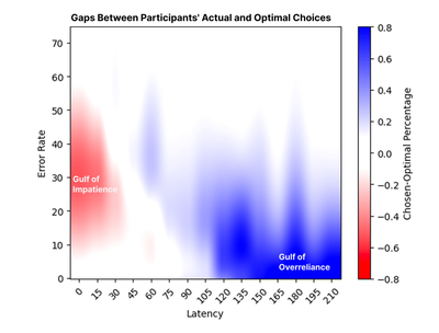
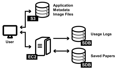
![Figure 8: Four plots illustrating key patterns in chosen versus optimal percentages of using Assisted Fill given various latency conditions. The y-axis in each chart represents the percentage of participants choosing Assisted Fill, with y = 1 meaning everyone chose Assisted Fill and y = 0 indicating no one chose Assisted Fill. The x-axis represents the different error rate conditions. The four horizontal charts represent these variables for increasing latency: 0s (top left), 30s (top right), 105s (bottom left), and 210s (bottom right). Sigmoid curves are fitted to the raw data to illustrate trends. Shaded areas around the red and blue curves represent 1-sigma bootstrap confidence intervals [8, 40].](/publication/to-use-or-not-to-use-impatience-and/figure-8-cropped_hu_3ad39be38217046.png)
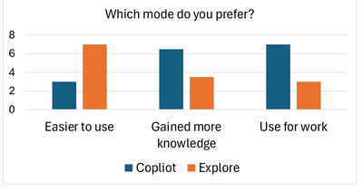
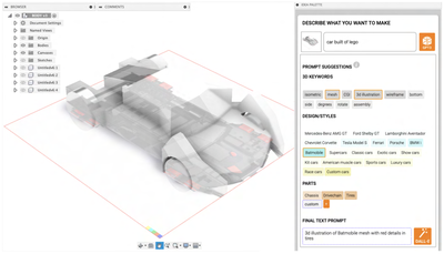
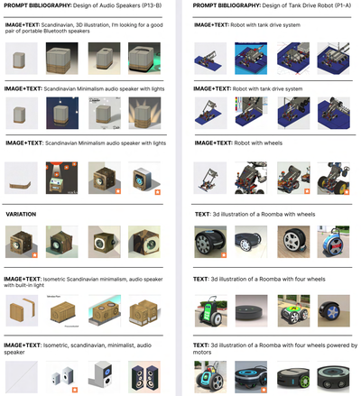
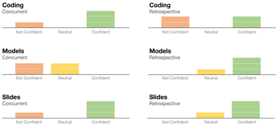
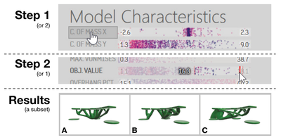
![Figure 11: For each respective mode, (a) average participant ratings [0-5] on their confidence in the designs generated and (b) number of participants who found a feasible solution that met all requirement metrics.](/publication/transformer-based-interfaces-for-mechanical-assembly-design-a/figure-11-cropped_hu_52f29f8bbc7ed828.png)
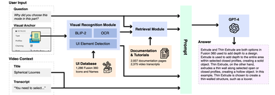
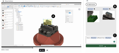
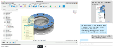
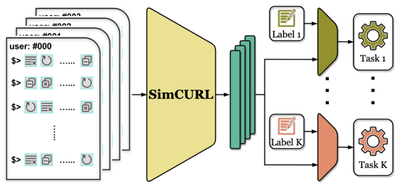
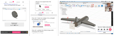
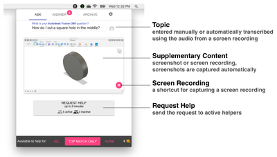
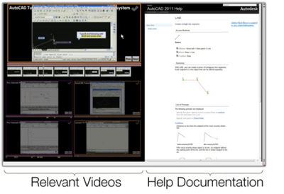
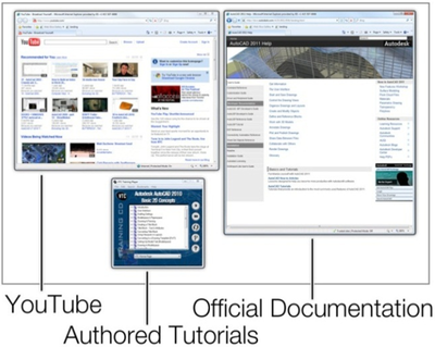
![Figure 4: Our Visual Recognition Module is composed of Image Captioning, UI Element Detection, and Optical CharacterRecognition (OCR). We use BLIP-2 [34] to obtain a general description of the visual](/publication/aqua-automated-question-answering-in-software-tutorial-videos/figure-4-cropped_hu_dff5115716a7ca2a.png)
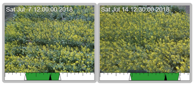
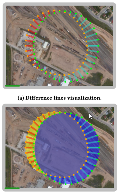


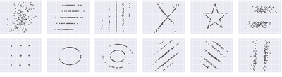
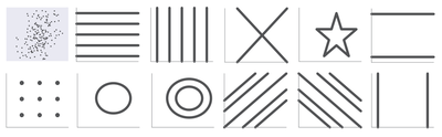
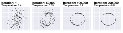
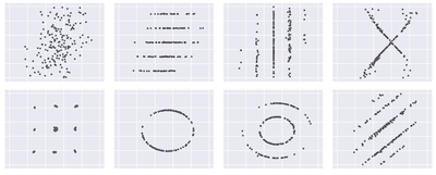
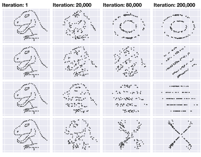
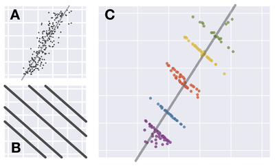
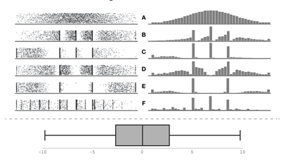
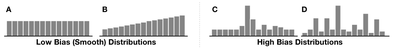
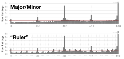
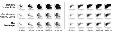
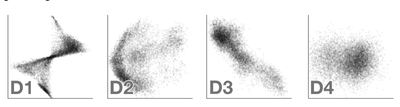
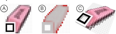
![Figure 8. Example of creating a “mirror” dataset as in [8].](/publication/same-stats/figure-9-cropped_hu_d7920ff0a08d2a85.png)


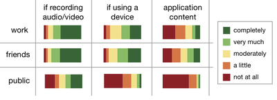
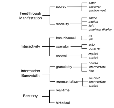
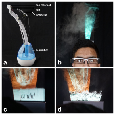
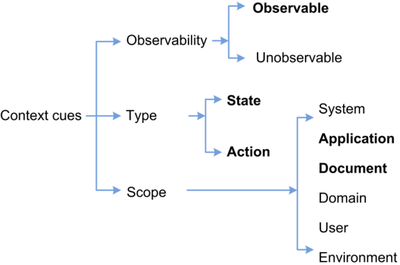
![Figure 2. Relationship of candid interaction to other types of social interaction in dimensions of Reeves et al. [35].](/publication/candid-interaction/figure-2-cropped_hu_9b34b479b20bee7f.png)


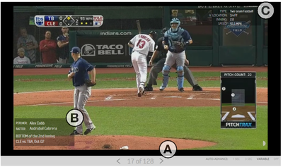
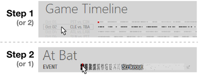


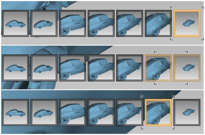
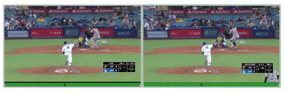
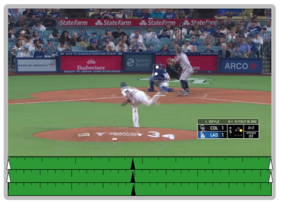
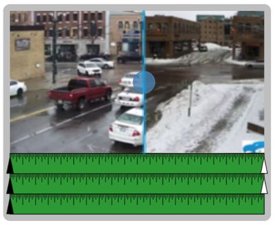
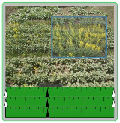
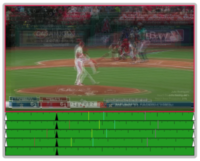
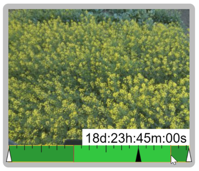
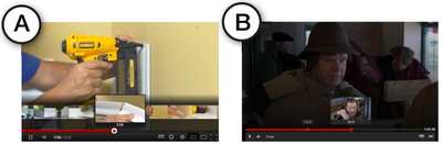
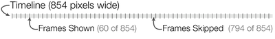
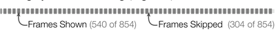
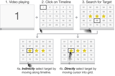
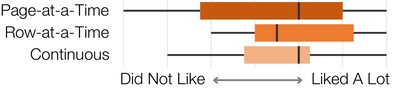
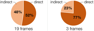
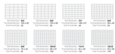
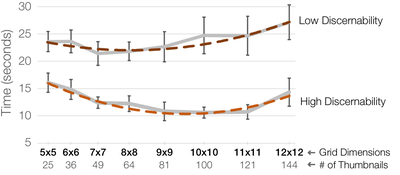
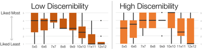
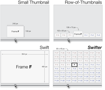
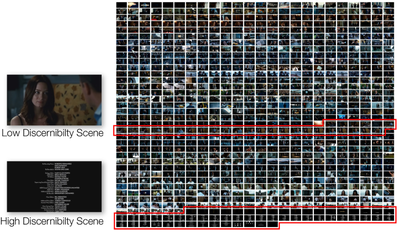
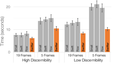
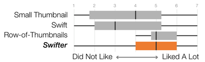
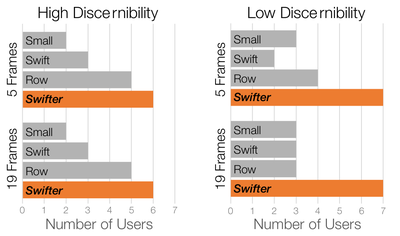
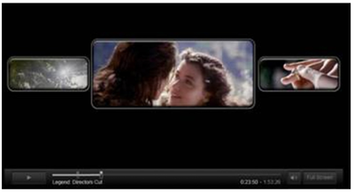
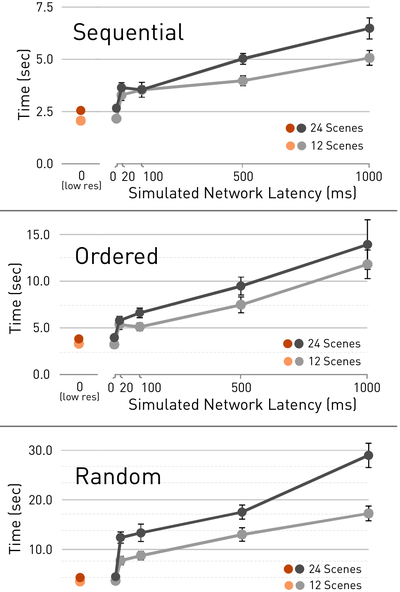
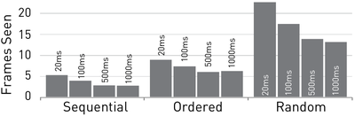
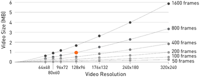
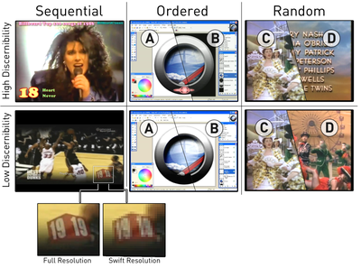
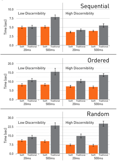
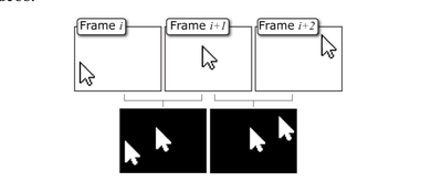
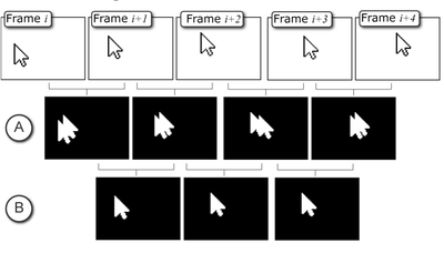
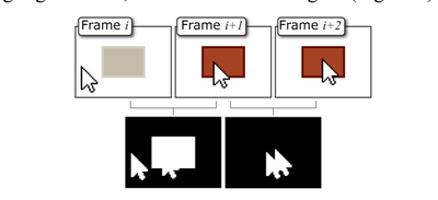
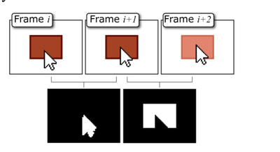
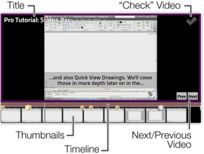
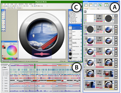
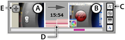
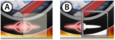
![Figure 1. Scrubbing behavior of a traditional streaming video player, the Swift interface [16], and our new Swifter interface, which shows multiple frames around the active timeline location and allows for direct selection of each frame.](/publication/swifter/figure-1-cropped_hu_9f41d6302edb8040.png)
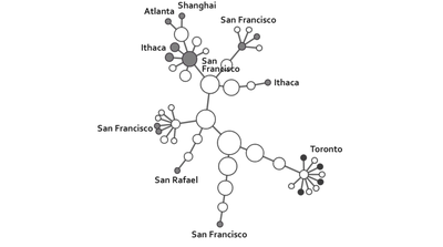
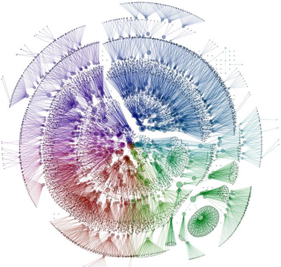
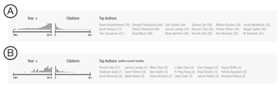
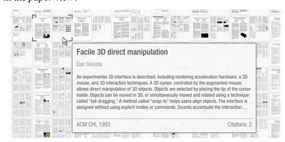
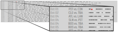
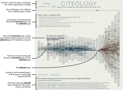
![Figure 1. Citeology for Spotlight [9]. (Note: high resolution vector version in Appendix A)](/publication/citeology/figure-1-cropped_hu_7393f9dcf37f2540.png)
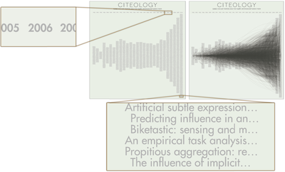
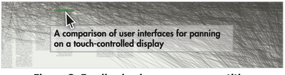
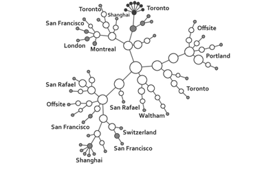
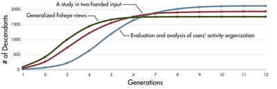
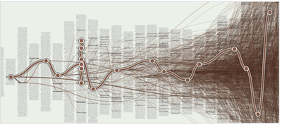
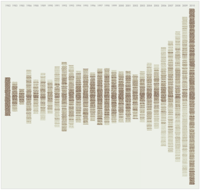
![Figure 4. Citeologies showing 1, 2, and All generations from the CHI 1995 paper Bricks: laying the foundations for graspable user interfaces [5].](/publication/citeology/figure-4-cropped_hu_d5263f13155d50b0.png)


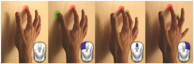
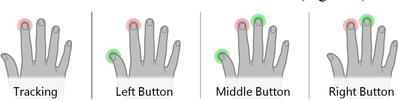
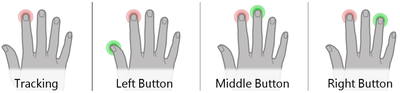
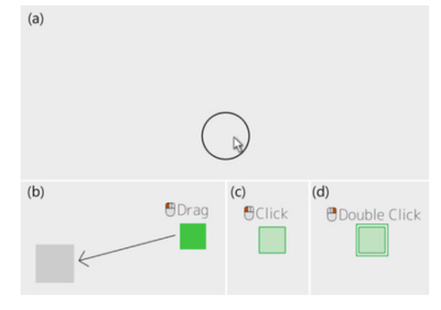
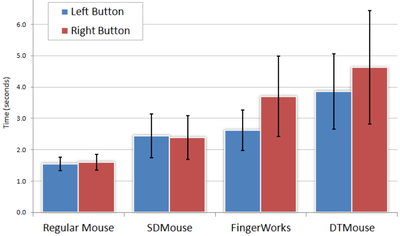
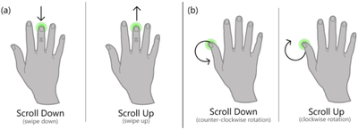
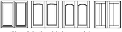
![Figure 5c]. Bymouse button wone could deteused.](/publication/ambient-help/figure-5-cropped_hu_5c46567a3f989575.png)
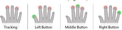
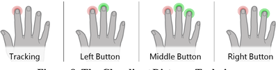
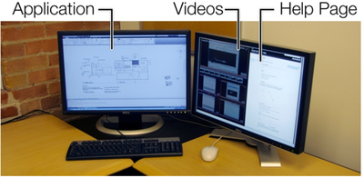
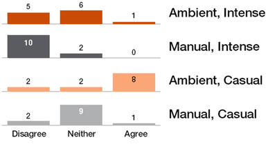
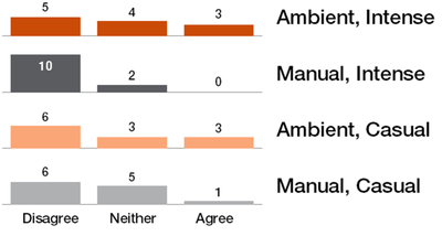
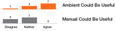
![Figure 11]. categories: (6, 7). The he ambient only 1 user](/publication/ambient-help/figure-9-cropped_hu_dfcafdde4a7fcfc0.png)


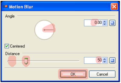
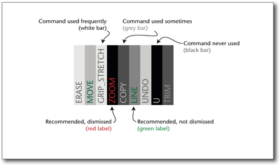
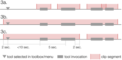
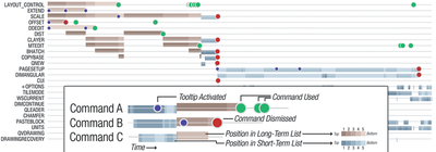
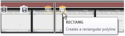
![Figure 10. When the cursor hovers over the ellipse tool event marker, previous setting events which effected that tool are highlighted. A halo [3] indicates the existence of an additional relevant set](/publication/chronicle/figure-10-cropped_hu_1b80c7bc4d102c88.png)